前提
- 入力層ニューロン 2つ
- 中間層ニューロン 6つ
- 出力層ニューロン 2つ
- 中間層の活性化関数:シグモイド関数
- 出力層の活性化関数:ソフトマックス関数
- 損失関数:交差エントロピー誤差
- 最適化アルゴリズム:確率的勾配降下法
- バッチサイズ:1
正解は0,1もしくは1,0のone-hotで表現しています。
ソースコード
%matplotlib inline
import numpy as np
import matplotlib.pyplot as plt
# -- 座標 --
X = np.arange(-1.0, 1.1, 0.1)
Y = np.arange(-1.0, 1.1, 0.1)
# -- 入力、正解データを作成 --
input_data = []
correct_data = []
for x in X:
for y in Y:
input_data.append([x, y])
if y < np.sin(np.pi * x): # y座標がsinカーブよりも下であれば
correct_data.append([0, 1]) # 下の領域
else:
correct_data.append( ) # 上の領域
n_data = len(correct_data) # データ数
input_data = np.array(input_data)
correct_data = np.array(correct_data)
# -- 各設定値 --
n_in = 2 # 入力層のニューロン数
n_mid = 6 # 中間層のニューロン数
n_out = 2 # 出力層のニューロン数
wb_width = 0.01 # 重みとバイアスの広がり具合
eta = 0.1 # 学習係数
epoch = 101
interval = 10 # 経過の表示間隔
# -- 中間層 --
class MiddleLayer:
def __init__(self, n_upper, n):
self.w = wb_width * np.random.randn(n_upper, n) # 重み(行列)
self.b = wb_width * np.random.randn(n) # バイアス(ベクトル)
def forward(self, x):
self.x = x
u = np.dot(x, self.w) + self.b
self.y = 1/(1+np.exp(-u)) # シグモイド関数
def backward(self, grad_y):
delta = grad_y * (1-self.y)*self.y
self.grad_w = np.dot(self.x.T, delta)
self.grad_b = np.sum(delta, axis=0)
self.grad_x = np.dot(delta, self.w.T)
def update(self, eta):
self.w -= eta * self.grad_w
self.b -= eta * self.grad_b
# -- 出力層 --
class OutputLayer:
def __init__(self, n_upper, n):
self.w = wb_width * np.random.randn(n_upper, n) # 重み(行列)
self.b = wb_width * np.random.randn(n) # バイアス(ベクトル)
def forward(self, x):
self.x = x
u = np.dot(x, self.w) + self.b
self.y = np.exp(u)/np.sum(np.exp(u), axis=1, keepdims=True) # ソフトマックス関数
def backward(self, t):
delta = self.y - t
self.grad_w = np.dot(self.x.T, delta)
self.grad_b = np.sum(delta, axis=0)
self.grad_x = np.dot(delta, self.w.T)
def update(self, eta):
self.w -= eta * self.grad_w
self.b -= eta * self.grad_b
# -- 各層の初期化 --
middle_layer = MiddleLayer(n_in, n_mid)
output_layer = OutputLayer(n_mid, n_out)
# -- 学習 --
sin_data = np.sin(np.pi * X) # 結果の検証用
for i in range(epoch):
# インデックスをシャッフル
index_random = np.arange(n_data)
np.random.shuffle(index_random)
# 結果の表示用
total_error = 0
x_1 = []
y_1 = []
x_2 = []
y_2 = []
for idx in index_random:
x = input_data[idx]
t = correct_data[idx]
# 順伝播
middle_layer.forward(x.reshape(1,2))
output_layer.forward(middle_layer.y)
# 逆伝播
output_layer.backward(t.reshape(1,2))
middle_layer.backward(output_layer.grad_x)
# 重みとバイアスの更新
middle_layer.update(eta)
output_layer.update(eta)
if i%interval == 0:
y = output_layer.y.reshape(-1) # 行列をベクトルに戻す
# 誤差の計算
total_error += - np.sum(t * np.log(y + 1e-7)) # 交差エントロピー誤差
# 確率の大小を比較し、分類する
if y[0] > y:
x_1.append(x[0])
y_1.append(x)
else:
x_2.append(x[0])
y_2.append(x)
if i%interval == 0:
# 出力のグラフ表示
plt.plot(X, sin_data, linestyle="dashed")
plt.scatter(x_1, y_1, marker="+")
plt.scatter(x_2, y_2, marker="x")
plt.show()
# エポック数と誤差の表示
print("Epoch:" + str(i) + "/" + str(epoch), "Error:" + str(total_error/n_data))
) # 上の領域
n_data = len(correct_data) # データ数
input_data = np.array(input_data)
correct_data = np.array(correct_data)
# -- 各設定値 --
n_in = 2 # 入力層のニューロン数
n_mid = 6 # 中間層のニューロン数
n_out = 2 # 出力層のニューロン数
wb_width = 0.01 # 重みとバイアスの広がり具合
eta = 0.1 # 学習係数
epoch = 101
interval = 10 # 経過の表示間隔
# -- 中間層 --
class MiddleLayer:
def __init__(self, n_upper, n):
self.w = wb_width * np.random.randn(n_upper, n) # 重み(行列)
self.b = wb_width * np.random.randn(n) # バイアス(ベクトル)
def forward(self, x):
self.x = x
u = np.dot(x, self.w) + self.b
self.y = 1/(1+np.exp(-u)) # シグモイド関数
def backward(self, grad_y):
delta = grad_y * (1-self.y)*self.y
self.grad_w = np.dot(self.x.T, delta)
self.grad_b = np.sum(delta, axis=0)
self.grad_x = np.dot(delta, self.w.T)
def update(self, eta):
self.w -= eta * self.grad_w
self.b -= eta * self.grad_b
# -- 出力層 --
class OutputLayer:
def __init__(self, n_upper, n):
self.w = wb_width * np.random.randn(n_upper, n) # 重み(行列)
self.b = wb_width * np.random.randn(n) # バイアス(ベクトル)
def forward(self, x):
self.x = x
u = np.dot(x, self.w) + self.b
self.y = np.exp(u)/np.sum(np.exp(u), axis=1, keepdims=True) # ソフトマックス関数
def backward(self, t):
delta = self.y - t
self.grad_w = np.dot(self.x.T, delta)
self.grad_b = np.sum(delta, axis=0)
self.grad_x = np.dot(delta, self.w.T)
def update(self, eta):
self.w -= eta * self.grad_w
self.b -= eta * self.grad_b
# -- 各層の初期化 --
middle_layer = MiddleLayer(n_in, n_mid)
output_layer = OutputLayer(n_mid, n_out)
# -- 学習 --
sin_data = np.sin(np.pi * X) # 結果の検証用
for i in range(epoch):
# インデックスをシャッフル
index_random = np.arange(n_data)
np.random.shuffle(index_random)
# 結果の表示用
total_error = 0
x_1 = []
y_1 = []
x_2 = []
y_2 = []
for idx in index_random:
x = input_data[idx]
t = correct_data[idx]
# 順伝播
middle_layer.forward(x.reshape(1,2))
output_layer.forward(middle_layer.y)
# 逆伝播
output_layer.backward(t.reshape(1,2))
middle_layer.backward(output_layer.grad_x)
# 重みとバイアスの更新
middle_layer.update(eta)
output_layer.update(eta)
if i%interval == 0:
y = output_layer.y.reshape(-1) # 行列をベクトルに戻す
# 誤差の計算
total_error += - np.sum(t * np.log(y + 1e-7)) # 交差エントロピー誤差
# 確率の大小を比較し、分類する
if y[0] > y:
x_1.append(x[0])
y_1.append(x)
else:
x_2.append(x[0])
y_2.append(x)
if i%interval == 0:
# 出力のグラフ表示
plt.plot(X, sin_data, linestyle="dashed")
plt.scatter(x_1, y_1, marker="+")
plt.scatter(x_2, y_2, marker="x")
plt.show()
# エポック数と誤差の表示
print("Epoch:" + str(i) + "/" + str(epoch), "Error:" + str(total_error/n_data))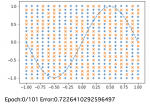
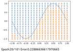
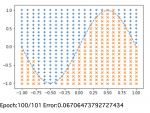
エポック数を重ねるとsinカーブの上下に各座標を正しく分類できるようになっていくことが確認できます。